
How to Create a Small Language Model from Scratch: Architecture, Training & Deployment
Master how to build, train, and deploy a small language model from scratch. Explore GQA, RoPE, synthetic data pipelines, PyTorch code, and GGUF quantization.
Deploying multi-billion-parameter language models for edge computing, local agent routing, and privacy-sensitive data workflows creates major operational bottlenecks. Massive cloud models incur heavy round-trip network latency, high inference fees, and excessive memory overhead on local hardware. Engineering teams need compact, task-specialized architectures that deliver frontier-grade reasoning inside strict resource budgets.
Learning how to create a small language model from scratch gives developers direct control over token efficiency, latency, and deployment costs. By combining modern architectural primitives with high-density synthetic data, a compact 1B to 3B parameter model can match or exceed legacy 7B baselines while running entirely in local memory.
Key Takeaways
- Modern small language models standardize on decoder-only Transformers equipped with Grouped-Query Attention (GQA), Rotary Position Embeddings (RoPE), RMSNorm, and SwiGLU feed-forward networks.
- Overtraining compact architectures on 1 to 5 trillion tokens of curated synthetic and educational text breaks classical chinchilla scaling limits to maximize runtime inference efficiency.
- Data quality overrides data volume; integrating synthetic textbook corpora like Cosmopedia v2 and FineWeb-Edu enables small models to surpass larger models on domain reasoning.
- Exporting trained weights to 4-bit GGUF formats reduces active memory footprints below 2GB VRAM, unlocking sub-30ms token latencies on consumer GPUs and edge microservers.
What Is a Small Language Model and Why Train One from Scratch
A small language model is a specialized neural network containing between 100 million and 4 billion parameters designed for high-throughput, low-latency execution. Unlike monolithic foundation models that require datacenter clusters, small language models execute on single consumer graphics cards, developer laptops, and embedded edge devices.
Historically, organizations deployed massive cloud APIs for basic classification, structured extraction, and tool routing tasks. As explored in our breakdown of cloud vs local AI architectures, executing repetitive agentic loops against remote cloud endpoints introduces substantial latency and compounding token expenses. Running a local model resolves these friction points.
Custom pre-training provides four concrete engineering advantages over relying strictly on public API endpoints:
- Deterministic Latency Profiles: Compact models eliminate variable wide-area network delays, delivering consistent sub-50ms token generation.
- Complete Data Sovereignty: Proprietary enterprise datasets, customer records, and codebases remain contained entirely within private infrastructure boundaries.
- Domain Vocabulary Alignment: Training a custom Byte-Pair Encoding (BPE) tokenizer avoids excessive token fragmentation on niche code syntaxes or medical nomenclatures.
- Permanent Offline Execution: Autonomous edge systems, robotics, and industrial appliances operate reliably without persistent internet access.
For teams building on-premise inference stacks, hosting custom weights locally requires selecting an appropriate runtime container and memory paging strategy. Custom-trained weights integrate directly into these execution environments.
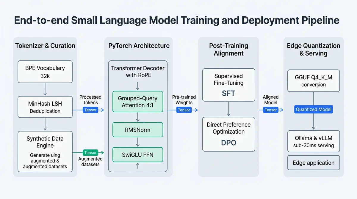 Figure 1: Complete end-to-end small language model pipeline spanning data synthesis, PyTorch pre-training, and quantized edge deployment.
Modern SLM Architecture: RoPE, GQA, SwiGLU, and RMSNorm
Building a modern small language model requires moving beyond early Transformer implementations. The open-source research ecosystem has converged on an optimized architectural standard that maximizes parameter expressiveness while minimizing inference memory overhead.
Modern architectures abandon standard Multi-Head Attention (MHA) and traditional LayerNorm in favor of four core components:
1. Grouped-Query Attention (GQA)
Standard Multi-Head Attention maintains separate Key and Value heads for every Query head. This creates massive Key-Value (KV) cache memory footprints that quickly exhaust device VRAM during long-context generation.
Grouped-query attention groups multiple query heads to share a single key-value projection head. In an 8:1 query-to-KV ratio, the memory bandwidth required to fetch cached activations drops by up to 8x. This optimization enables a 2B parameter model to handle 16K token context windows on standard consumer hardware without out-of-memory crashes.
2. Rotary Position Embeddings (RoPE)
Absolute positional embeddings assign static positional vectors to input tokens, preventing models from extrapolating past their initial training length. Rotary position embeddings incorporate position information directly into query and key representations via rotation matrices in complex coordinate space.
RoPE preserves relative token distances naturally through inner products. By scaling the base frequency parameter (theta) during mid-training, engineers can double or quadruple effective context lengths with minimal loss in model perplexity.
3. Root Mean Square Normalization (RMSNorm)
Standard LayerNorm calculates both the mean and variance across activation dimensions to normalize layer inputs. This introduces dual reduction operations that slow down memory throughput.
RMSNorm modifies this equation by normalizing solely by the root mean square of activation inputs, omitting the mean-centering step:
$$\text{RMSNorm}(x) = \frac{x}{\sqrt{\frac{1}{d} \sum_{i=1}^d x_i^2 + \epsilon}} \odot \gamma$$
Evaluating RMSNorm vs LayerNorm demonstrates that omitting the mean calculation preserves normalization stability while yielding a 10% to 25% training speed improvement across GPU kernels.
4. SwiGLU Activation Function
Traditional feed-forward networks (FFN) apply ReLU or GELU activations across intermediate projections. Modern small models employ SwiGLU, a gated activation function combining the Swish function with a bilinear projection:
$$\text{SwiGLU}(x) = (\text{Swish}(xW) \otimes xV) W_2$$
While the swiglu activation function requires three linear weight matrices instead of two, empirical benchmarks consistently demonstrate that SwiGLU delivers significantly better parameter efficiency than standard GELU networks.
| Model Tier | Parameter Range | Target Pre-Training Tokens | KV Cache per 4K Context (MHA vs GQA) | 4-bit Quantized VRAM | Production Workload Target |
|---|---|---|---|---|---|
| Edge Micro | 135M to 360M | 500B to 2 Trillion | 256MB vs 32MB | 250MB to 450MB | Embedded microcontrollers, edge sensors, intent routing |
| Mobile Compact | 1.5B to 2.0B | 2 Trillion to 11 Trillion | 1.2GB vs 150MB | 1.2GB to 1.8GB | Mobile devices, local coding copilots, private agent tools |
| High Reasoning | 3.0B to 4.0B | 3 Trillion to 8 Trillion | 2.4GB vs 300MB | 2.2GB to 3.1GB | Complex logic extraction, mathematical reasoning, agent nodes |
| Workstation Engine | 7.0B to 9.0B | 5 Trillion to 15 Trillion | 4.8GB vs 600MB | 4.8GB to 6.2GB | Autonomous engineering workflows, multi-document synthesis |
As reflected in our analysis of the best open-source LLMs, models utilizing GQA and high-ratio token overtraining represent the frontier of efficient local inference.
Data Curation Pipeline: Synthetic Textbooks and Token Mixes
Modern small language model performance depends primarily on dataset quality rather than raw parameter scale. Early foundation models relied on indiscriminate web scrapes like uncleaned Common Crawl, which introduced duplicate text, forum arguments, and low-information noise into pre-training batches.
The release of models like Hugging Face SmolLM2 and Microsoft Phi-4 proved that synthetic educational content allows compact models to outperform larger architectures. As detailed in the Hugging Face SmolLM2 Architecture and Cosmopedia v2 Dataset, overtraining a 1.7B parameter network on 11 trillion curated educational tokens achieves a 68.7% HellaSwag benchmark score, outperforming classical models with several times its parameter footprint.
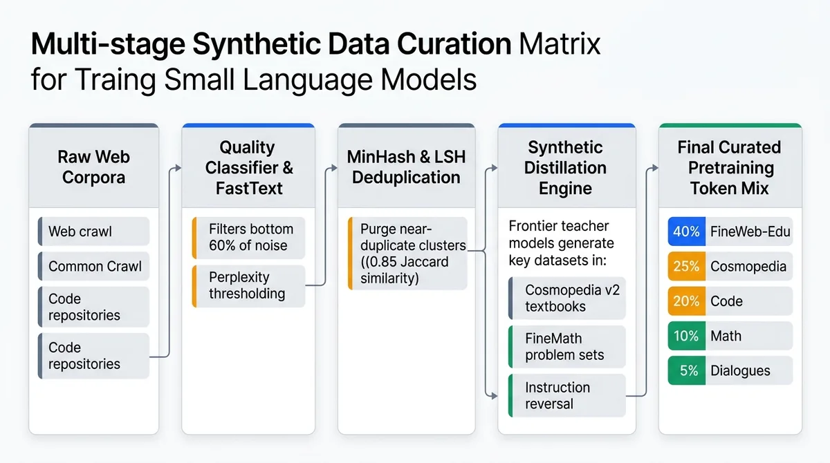 Figure 2: Multi-stage data curation pipeline filtering web crawls into high-density educational datasets alongside frontier synthetic generation.
A production synthetic data pipeline follows four sequential stages:
Stage 1: Quality Classifier Filtering
Raw web documents pass through fast text classifiers trained on high-standard benchmarks such as Wikipedia, arXiv papers, and curated textbooks. FastText models score incoming documents for perplexity, grammatical density, and technical depth, discarding the lowest 60% of organic web text.
Stage 2: Deduplication and MinHash LSH
Duplicate documents distort language model priors and encourage rote memorization over generalized reasoning. Using MinHash with Locality Sensitive Hashing (LSH), data pipelines identify and purge near-identical document clusters at a 0.85 Jaccard similarity threshold.
Stage 3: Frontier Synthetic Generation
Following principles established in the Microsoft Research Phi-4 Technical Report on arXiv, teams leverage frontier models to transform raw source material into high-density educational exercises. High-capability teacher models rewrite dry documentation into interactive problem sets, code walkthroughs, and step-by-step reasoning dialogues.
Synthetic generation workflows enforce techniques like Instruction Reversal and Partial Answer Masking (PAM) to verify that generated data emphasizes step-by-step logic over shallow pattern matching.
Stage 4: Balanced Pre-Training Token Recipe
A robust, general-purpose small model pre-training mix allocates tokens across distinct knowledge domains:
- Curated Educational Web (FineWeb-Edu): 40%
- Synthetic Textbooks & Reasoning Exercises (Cosmopedia v2): 25%
- Permissive Open-Source Code (The Stack v2 / StarCoder): 20%
- Mathematical Problem Sets (FineMath / OpenWebMath): 10%
- High-Standard Conversational Dialogues (SmolTalk): 5%
Training a Custom Byte-Pair Encoding (BPE) Tokenizer
Before feeding text into neural networks, engineers must train a custom tokenizer to compress domain text efficiently. The following script uses the Hugging Face tokenizers library to build a 32,000-token ByteLevel BPE tokenizer complete with ChatML special tokens:
from tokenizers import Tokenizer, decoders, models, normalizers, pre_tokenizers, trainers

def train_custom_bpe_tokenizer(corpus_files: list[str], vocab_size: int = 32000) -> Tokenizer:
    """Train a ByteLevel Byte-Pair Encoding tokenizer with ChatML tokens."""
    tokenizer = Tokenizer(models.BPE(unk_token="<|unk|>"))
    tokenizer.normalizer = normalizers.NFKC()
    tokenizer.pre_tokenizer = pre_tokenizers.ByteLevel(add_prefix_space=False)
    tokenizer.decoder = decoders.ByteLevel()

    special_tokens = ["<|endoftext|>", "<|im_start|>", "<|im_end|>", "<|unk|>"]
    trainer = trainers.BpeTrainer(
        vocab_size=vocab_size,
        special_tokens=special_tokens,
        initial_alphabet=pre_tokenizers.ByteLevel.alphabet(),
    )

    tokenizer.train(corpus_files, trainer)
    tokenizer.save("tokenizer.json")
    return tokenizer
Step-by-Step Pre-Training Implementation in PyTorch
Pre-training a small language model requires implementing the core architecture using typed PyTorch tensors. Below is a complete, modular implementation of a modern Transformer decoder block incorporating RMSNorm, RoPE, Grouped-Query Attention, and SwiGLU activations.
import math
from dataclasses import dataclass
from typing import Optional, Tuple
import torch
import torch.nn as nn
import torch.nn.functional as F

@dataclass
class SLMConfig:
    vocab_size: int = 32000
    hidden_dim: int = 2048
    intermediate_dim: int = 5632
    num_layers: int = 24
    num_query_heads: int = 16
    num_kv_heads: int = 4  # 4:1 GQA ratio
    max_position_embeddings: int = 4096
    rope_theta: float = 10000.0
    rms_norm_eps: float = 1e-6

class RMSNorm(nn.Module):
    """Root Mean Square Layer Normalization without mean subtraction."""
    def __init__(self, dim: int, eps: float = 1e-6):
        super().__init__()
        self.eps = eps
        self.weight = nn.Parameter(torch.ones(dim))

    def forward(self, x: torch.Tensor) -> torch.Tensor:
        variance = x.pow(2).mean(-1, keepdim=True)
        normed = x * torch.rsqrt(variance + self.eps)
        return normed * self.weight

class RotaryEmbedding(nn.Module):
    """Rotary Position Embedding (RoPE) for relative positional encoding."""
    def __init__(self, dim: int, max_seq_len: int = 4096, theta: float = 10000.0):
        super().__init__()
        self.dim = dim
        inv_freq = 1.0 / (theta ** (torch.arange(0, dim, 2).float() / dim))
        self.register_buffer("inv_freq", inv_freq, persistent=False)

        t = torch.arange(max_seq_len, dtype=torch.float32)
        freqs = torch.outer(t, self.inv_freq)
        emb = torch.cat((freqs, freqs), dim=-1)
        self.register_buffer("cos_cached", emb.cos(), persistent=False)
        self.register_buffer("sin_cached", emb.sin(), persistent=False)

    def forward(self, x: torch.Tensor, seq_len: int) -> Tuple[torch.Tensor, torch.Tensor]:
        return self.cos_cached[:seq_len, :], self.sin_cached[:seq_len, :]

def rotate_half(x: torch.Tensor) -> torch.Tensor:
    x1 = x[..., : x.shape[-1] // 2]
    x2 = x[..., x.shape[-1] // 2 :]
    return torch.cat((-x2, x1), dim=-1)

def apply_rotary_pos_emb(q: torch.Tensor, k: torch.Tensor, cos: torch.Tensor, sin: torch.Tensor) -> Tuple[torch.Tensor, torch.Tensor]:
    cos = cos.unsqueeze(0).unsqueeze(0)  # [1, 1, seq_len, head_dim]
    sin = sin.unsqueeze(0).unsqueeze(0)
    q_embed = (q * cos) + (rotate_half(q) * sin)
    k_embed = (k * cos) + (rotate_half(k) * sin)
    return q_embed, k_embed

class GroupedQueryAttention(nn.Module):
    """Grouped-Query Attention with shared Key-Value projection heads."""
    def __init__(self, config: SLMConfig):
        super().__init__()
        self.num_query_heads = config.num_query_heads
        self.num_kv_heads = config.num_kv_heads
        self.head_dim = config.hidden_dim // config.num_query_heads
        self.num_queries_per_kv = self.num_query_heads // self.num_kv_heads

        self.q_proj = nn.Linear(config.hidden_dim, config.num_query_heads * self.head_dim, bias=False)
        self.k_proj = nn.Linear(config.hidden_dim, self.num_kv_heads * self.head_dim, bias=False)
        self.v_proj = nn.Linear(config.hidden_dim, self.num_kv_heads * self.head_dim, bias=False)
        self.out_proj = nn.Linear(config.num_query_heads * self.head_dim, config.hidden_dim, bias=False)

    def forward(self, x: torch.Tensor, cos: torch.Tensor, sin: torch.Tensor, mask: Optional[torch.Tensor] = None) -> torch.Tensor:
        batch_size, seq_len, _ = x.shape

        q = self.q_proj(x).view(batch_size, seq_len, self.num_query_heads, self.head_dim).transpose(1, 2)
        k = self.k_proj(x).view(batch_size, seq_len, self.num_kv_heads, self.head_dim).transpose(1, 2)
        v = self.v_proj(x).view(batch_size, seq_len, self.num_kv_heads, self.head_dim).transpose(1, 2)

        q, k = apply_rotary_pos_emb(q, k, cos, sin)

        # Expand KV heads to match query heads for grouped computation
        if self.num_queries_per_kv > 1:
            k = k.repeat_interleave(self.num_queries_per_kv, dim=1)
            v = v.repeat_interleave(self.num_queries_per_kv, dim=1)

        scores = torch.matmul(q, k.transpose(-2, -1)) / math.sqrt(self.head_dim)
        if mask is not None:
            scores = scores + mask

        attn_weights = F.softmax(scores, dim=-1)
        output = torch.matmul(attn_weights, v)
        output = output.transpose(1, 2).contiguous().view(batch_size, seq_len, -1)
        return self.out_proj(output)

class SwiGLUMLP(nn.Module):
    """SwiGLU feed-forward layer with gated bilinear projection."""
    def __init__(self, hidden_dim: int, intermediate_dim: int):
        super().__init__()
        self.gate_proj = nn.Linear(hidden_dim, intermediate_dim, bias=False)
        self.up_proj = nn.Linear(hidden_dim, intermediate_dim, bias=False)
        self.down_proj = nn.Linear(intermediate_dim, hidden_dim, bias=False)

    def forward(self, x: torch.Tensor) -> torch.Tensor:
        return self.down_proj(F.silu(self.gate_proj(x)) * self.up_proj(x))

class SLMDecoderBlock(nn.Module):
    """Complete Transformer Decoder Block with pre-normalization."""
    def __init__(self, config: SLMConfig):
        super().__init__()
        self.input_norm = RMSNorm(config.hidden_dim, config.rms_norm_eps)
        self.self_attn = GroupedQueryAttention(config)
        self.post_attn_norm = RMSNorm(config.hidden_dim, config.rms_norm_eps)
        self.mlp = SwiGLUMLP(config.hidden_dim, config.intermediate_dim)

    def forward(self, x: torch.Tensor, cos: torch.Tensor, sin: torch.Tensor, mask: Optional[torch.Tensor] = None) -> torch.Tensor:
        normed_x = self.input_norm(x)
        attn_out = self.self_attn(normed_x, cos, sin, mask)
        x = x + attn_out
        x = x + self.mlp(self.post_attn_norm(x))
        return x
Complete Model Architecture and Autoregressive Generator
The decoder blocks integrate into a top-level causal language model. This class manages token embeddings, causal triangular attention masking, weight-tied output projections, and autoregressive text generation:
class SmallLanguageModel(nn.Module):
    """Complete causal language model with weight-tying and autoregressive generation."""
    def __init__(self, config: SLMConfig):
        super().__init__()
        self.config = config
        self.embed_tokens = nn.Embedding(config.vocab_size, config.hidden_dim)
        self.rope = RotaryEmbedding(config.hidden_dim // config.num_query_heads, config.max_position_embeddings, config.rope_theta)
        self.layers = nn.ModuleList([SLMDecoderBlock(config) for _ in range(config.num_layers)])
        self.norm = RMSNorm(config.hidden_dim, config.rms_norm_eps)
        self.lm_head = nn.Linear(config.hidden_dim, config.vocab_size, bias=False)

        # Tie embeddings to output projection matrix to save parameters
        self.lm_head.weight = self.embed_tokens.weight

    def forward(self, input_ids: torch.Tensor, labels: Optional[torch.Tensor] = None) -> Tuple[torch.Tensor, Optional[torch.Tensor]]:
        batch_size, seq_len = input_ids.shape
        x = self.embed_tokens(input_ids)
        cos, sin = self.rope(x, seq_len)

        # Causal triangular attention mask
        mask = torch.triu(torch.full((seq_len, seq_len), float("-inf"), device=input_ids.device), diagonal=1)
        mask = mask.unsqueeze(0).unsqueeze(0)

        for layer in self.layers:
            x = layer(x, cos, sin, mask)

        x = self.norm(x)
        logits = self.lm_head(x)

        loss = None
        if labels is not None:
            shift_logits = logits[..., :-1, :].contiguous()
            shift_labels = labels[..., 1:].contiguous()
            loss = F.cross_entropy(shift_logits.view(-1, self.config.vocab_size), shift_labels.view(-1))

        return logits, loss

    @torch.no_grad()
    def generate(self, input_ids: torch.Tensor, max_new_tokens: int = 50, temperature: float = 0.7, top_k: int = 50) -> torch.Tensor:
        """Autoregressive text generation with temperature and top-k filtering."""
        self.eval()
        for _ in range(max_new_tokens):
            idx_cond = input_ids if input_ids.size(1) <= self.config.max_position_embeddings else input_ids[:, -self.config.max_position_embeddings:]
            logits, _ = self(idx_cond)
            next_logits = logits[:, -1, :] / max(temperature, 1e-5)

            if top_k > 0:
                v, _ = torch.topk(next_logits, min(top_k, next_logits.size(-1)))
                next_logits[next_logits < v[:, [-1]]] = float("-inf")

            probs = F.softmax(next_logits, dim=-1)
            next_token = torch.multinomial(probs, num_samples=1)
            input_ids = torch.cat((input_ids, next_token), dim=1)

            if next_token.item() == 0:  # End of text token
                break
        return input_ids
Dataset Streaming and Sequence Packing
Pre-training requires packing multiple variable-length text records into contiguous sequences of 2,048 tokens. This eliminates padding waste and keeps GPU compute utilization at peak capacity:
from typing import Iterator
from datasets import load_dataset
from tokenizers import Tokenizer

def stream_and_pack_tokens(dataset_name: str, tokenizer: Tokenizer, seq_len: int = 2048) -> Iterator[torch.Tensor]:
    """Stream dataset and pack continuous tokens into fixed-length batches."""
    dataset = load_dataset(dataset_name, split="train", streaming=True)
    buffer = []

    for item in dataset:
        tokens = tokenizer.encode(item["text"]).ids + [0]  # Append <|endoftext|>
        buffer.extend(tokens)

        while len(buffer) >= seq_len:
            chunk = buffer[:seq_len]
            buffer = buffer[seq_len:]
            yield torch.tensor(chunk, dtype=torch.long)
Complete Pre-Training Execution Script
The complete pre-training execution pipeline initializes the model, configures AdamW optimization, and executes gradient-clipped training steps using bfloat16 mixed precision:
from torch.optim import AdamW
from torch.optim.lr_scheduler import CosineAnnealingLR

def configure_optimizers(model: nn.Module):
    """Configure modern AdamW optimizer and cosine schedule."""
    decay_params = [p for n, p in model.named_parameters() if p.dim() >= 2]
    no_decay_params = [p for n, p in model.named_parameters() if p.dim() < 2]

    optim_groups = [
        {"params": decay_params, "weight_decay": 0.1},
        {"params": no_decay_params, "weight_decay": 0.0},
    ]

    optimizer = AdamW(optim_groups, lr=3e-4, betas=(0.9, 0.95), eps=1e-8)
    scheduler = CosineAnnealingLR(optimizer, T_max=100000, eta_min=3e-5)
    return optimizer, scheduler

def run_pretraining_loop(model: SmallLanguageModel, token_stream: Iterator[torch.Tensor], steps: int = 1000):
    """Complete minimal training loop with bfloat16 and gradient clipping."""
    device = "cuda" if torch.cuda.is_available() else "cpu"
    model.to(device)
    optimizer, scheduler = configure_optimizers(model)

    model.train()
    for step in range(steps):
        batch = next(token_stream).unsqueeze(0).to(device)
        optimizer.zero_grad(set_to_none=True)

        with torch.autocast(device_type=device, dtype=torch.bfloat16):
            _, loss = model(input_ids=batch, labels=batch)

        loss.backward()
        torch.nn.utils.clip_grad_norm_(model.parameters(), max_norm=1.0)
        optimizer.step()
        scheduler.step()

        if step % 100 == 0:
            print(f"Step {step}/{steps} | Loss: {loss.item():.4f}")

    torch.save(model.state_dict(), "slm_base_weights.pt")
Post-Training Alignment: SFT, DPO, and Exporting to GGUF
Pre-training yields a raw base model capable of predicting the next probable token, but it lacks instruction obedience and conversational alignment. Production readiness requires two targeted post-training phases followed by deployment quantization.
Phase 1: Supervised Fine-Tuning (SFT) with LoRA
The base model trains on 50,000 to 200,000 curated instruction-response pairs formatted in a standard chat template. Rather than training all weights, Low-Rank Adaptation (LoRA) trains lightweight adapter matrices over attention projections:
from trl import SFTTrainer, SFTConfig
from peft import LoraConfig

def execute_sft_alignment(model: nn.Module, train_dataset):
    """Execute Supervised Fine-Tuning with Low-Rank Adaptation (LoRA)."""
    peft_config = LoraConfig(
        r=16,
        lora_alpha=32,
        target_modules=["q_proj", "v_proj"],
        lora_dropout=0.05,
        bias="none",
        task_type="CAUSAL_LM",
    )

    training_args = SFTConfig(
        output_dir="./slm-instruct",
        learning_rate=2e-4,
        num_train_epochs=3,
        per_device_train_batch_size=4,
        gradient_accumulation_steps=4,
        fp16=True,
        logging_steps=10,
    )

    trainer = SFTTrainer(
        model=model,
        train_dataset=train_dataset,
        peft_config=peft_config,
        dataset_text_field="text",
        max_seq_length=2048,
        args=training_args,
    )
    trainer.train()
Phase 2: Direct Preference Optimization (DPO)
Traditional Reinforcement Learning from Human Feedback (RLHF) required training a separate reward model and managing unstable PPO loops. Applying direct preference optimization directly optimizes the language model on binary chosen versus rejected response pairs:
$$\mathcal{L}{\text{DPO}}(\theta; \pi{\text{ref}}) = -\mathbb{E}{(x, y_w, y_l)} \left[ \log \sigma \left( \beta \log \frac{\pi\theta(y_w \mid x)}{\pi_{\text{ref}}(y_w \mid x)} - \beta \log \frac{\pi_\theta(y_l \mid x)}{\pi_{\text{ref}}(y_l \mid x)} \right) \right]$$
Setting $\beta = 0.1$ prevents the policy network from diverging excessively from the reference model while penalizing verbose hallucinations and formatting errors.
Phase 3: Exporting to GGUF for llama.cpp and Ollama
Following alignment, weights are exported from PyTorch checkpoints into the GGUF binary format defined in the llama.cpp GGUF Quantization Specification on GitHub. Implementing GGUF quantization from FP16 weights to 4-bit medium precision (Q4_K_M) drops model memory footprints by over 70%:
# 1. Convert PyTorch / Hugging Face model directory to FP16 GGUF
python3 llama.cpp/convert_hf_to_gguf.py ./my-custom-slm-model \
    --outfile ./my-custom-slm.fp16.gguf \
    --outtype f16

# 2. Quantize FP16 weights to 4-bit Medium (Q4_K_M)
./llama.cpp/llama-quantize \
    ./my-custom-slm.fp16.gguf \
    ./my-custom-slm-q4km.gguf \
    q4_k_m

# 3. Create an Ollama Modelfile for local serving
cat << 'EOF' > Modelfile
FROM ./my-custom-slm-q4km.gguf
PARAMETER temperature 0.2
PARAMETER stop "<|im_end|>"
TEMPLATE """<|im_start|>system
{{ .System }}<|im_end|>
<|im_start|>user
{{ .Prompt }}<|im_end|>
<|im_start|>assistant
"""
EOF

# 4. Build and run locally via Ollama
ollama create custom-slm -f Modelfile
ollama run custom-slm "Analyze system log anomalies."
For embedded or low-power hardware, our tutorial on running local AI on a Raspberry Pi outlines memory paging configurations for running quantized SLM weights on 8GB single-board computers.
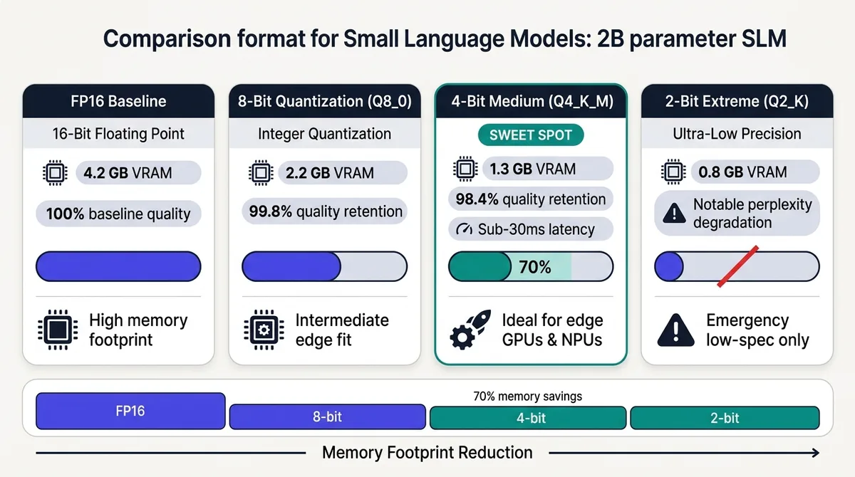 Figure 3: Memory footprint vs perplexity trade-offs across quantization profiles, highlighting Q4_K_M as the sweet spot for edge VRAM budgets.
Production Failure Modes, Loss Spikes, and Hardware Sizing
Training language models from scratch introduces complex systems failures that differ substantially from traditional software engineering bugs. Preparing for these failure modes before launching compute jobs protects engineering budgets and model weights.
Failure Mode 1: Mid-Training Loss Spikes
A common failure mode during pre-training is sudden loss divergence, where training loss spikes unpredictably after tens of thousands of stable steps. This issue is typically caused by activation outliers in attention projection layers or corrupted token batches.
[!WARNING] If a loss spike occurs, do not continue training from the corrupted state. Roll back the checkpoint to 1,000 steps prior to the anomaly, drop the global learning rate by 15%, and purge the corrupt data shards from the data streaming queue before resuming.
Failure Mode 2: Premature Perplexity Saturation
When models stop improving well before their target token budget, the cause is almost universally data repetition or synthetic model collapse. If synthetic text generated by the same teacher model lacks sufficient diversity, student networks quickly overfit on shallow lexical mannerisms.
Ensure synthetic generation prompts incorporate randomized temperatures, multi-seed scenarios, and diverse system personas to maintain high vocabulary entropy throughout all training epochs.
Hardware Sizing Guidelines
Sizing hardware correctly depends on whether the team is pre-training from scratch or executing post-training fine-tuning:
- Pre-Training from Scratch (1B to 2B Parameters): Pre-training a 1.5B model on 1 trillion tokens requires approximately 1,500 to 2,500 GPU hours on Nvidia H100 (80GB SXM5) nodes utilizing DeepSpeed ZeRO-2 or PyTorch FSDP.
- LoRA / QLoRA Fine-Tuning: Specializing a pre-trained small model on domain tasks requires only a single consumer GPU (RTX 4090 or Apple Silicon M-series chip with 24GB Unified Memory), completing in 2 to 6 hours.
- Local Inference Serving: A 4-bit quantized 2B model requires 1.8GB of VRAM and consumes under 15 watts of power on edge NPUs while generating over 80 tokens per second. For automated desktop orchestration and model management, reference our complete Ollama local AI deployment guide.
Frequently Asked Questions About Building Small Language Models
What parameter range qualifies as a small language model?
A small language model generally ranges between 100 million and 4 billion parameters. These models are engineered to run with full efficiency on single consumer GPUs, laptops, or edge appliances without requiring distributed cloud clusters.
How much data is required to train a small language model from scratch?
Modern state-of-the-art small language models require between 1 trillion and 5 trillion high-quality tokens to achieve strong reasoning and general language capabilities. Rather than adhering to compute-optimal Chinchilla thresholds, modern teams intentionally overtrain small models to maximize downstream inference efficiency.
Why is Grouped-Query Attention critical for small language models?
Grouped-Query Attention reduces Key-Value cache memory bandwidth requirements by sharing key and value heads across multiple query heads. This reduction enables compact models to handle long context windows on edge devices with strictly bounded memory.
Can you train a small language model on a single consumer GPU?
Pre-training an SLM from scratch typically requires a multi-GPU cluster or rented cloud instances for several days, though miniature 100M-parameter prototypes can run on a single RTX 4090. In contrast, fine-tuning an existing open SLM with LoRA or QLoRA easily executes on a single consumer GPU with 16GB of VRAM.