How LLMs Are Actually Trained: Pretraining, SFT & Post-Training Explained Step by Step
Explore how modern LLMs are trained step by step, covering massive pretraining on web tokens, supervised fine-tuning with loss masking, and preference alignment.
Understanding how are llms trained explained from first principles requires looking beneath the polished web interfaces of conversational chatbots. A finished artificial intelligence assistant is not a monolithic program written by software engineers, nor is it created in a single uninterrupted training loop.
Instead, modern frontier systems pass through a structured, multi-stage factory. Raw unstructured text converts into semantic representations, which are then refined through curated instruction sets and reinforced through behavioral constraints. If you are building on a foundational large language model architecture, knowing these distinct stages is essential for effective fine-tuning, system prompt engineering, and model evaluation.
Key Takeaways:
- Large language model training follows a strict three-stage pipeline: self-supervised pretraining on trillions of tokens, supervised fine-tuning (SFT) on curated dialogues, and reinforcement alignment.
- Pretraining consumes over 98% of total computational compute and establishes world knowledge through next-token prediction, but leaves the model as a document autocompleter.
- Supervised fine-tuning transforms raw base completions into structured conversational assistants by applying cross-entropy loss exclusively to assistant response tokens.
- Post-training alignment uses preference optimization (DPO, RLHF) and rule-based verification (GRPO) to steer safety, eliminate sycophancy, and unlock chain-of-thought reasoning.
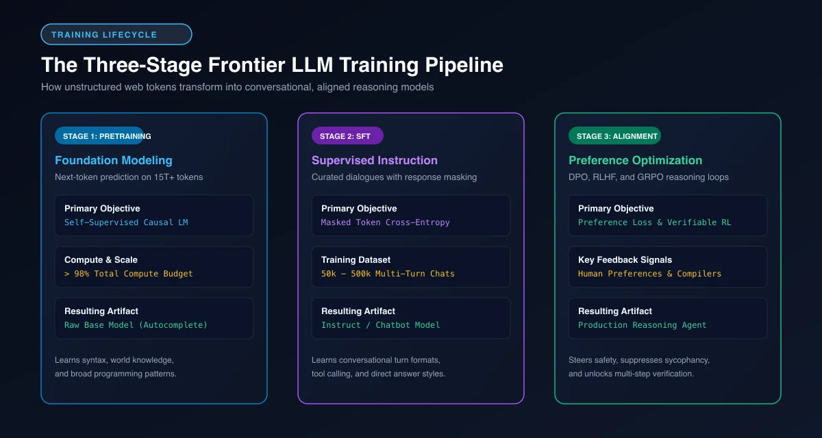 Figure 1: The three-stage frontier LLM training lifecycle from raw web corpus pretraining to supervised instruction tuning and post-training preference alignment.
The Three-Stage LLM Lifecycle Overview
Every state-of-the-art model today undergoes three sequential phases: pretraining, supervised fine-tuning (SFT), and post-training preference alignment. Each stage solves a completely different mathematical objective, uses different datasets, and demands vastly different computational budgets.
During Stage 1 (Pretraining), the model ingests massive web dumps, digitised books, academic papers, and source code repositories. The training objective is simple: given a sequence of tokens, predict the immediate next token through causal language modeling.
This stage creates a “base model” possessing deep linguistic competence and broad world knowledge, yet lacking conversational awareness. If you prompt a base model with “How do I bake bread?”, it might append “Chapter 4: Yeast Fermentation Techniques” instead of answering your question.
Stage 2 (Supervised Fine-Tuning) cures this autocomplete behavior. Engineers expose the base model to thousands of carefully formatted multi-turn conversations between a user and an ideal assistant. Through this process, the model learns the conversational turn format, system roles, and direct question-answering behavior.
Stage 3 (Post-Training Alignment) refines the model’s judgment, tone, and reasoning depth. Using algorithms like Direct Preference Optimization (DPO) and Group Relative Policy Optimization (GRPO), the model learns which candidate answers humans prefer and which mathematical reasoning steps lead to verifiable truths. Alternatively, compact student models can absorb these capabilities directly through knowledge distillation techniques without running massive reinforcement loops.
Stage 1: Pretraining and Next-Token Prediction at Scale
Pretraining is the most compute-intensive undertaking in modern computer science. It consumes between 98% and 99% of the entire lifecycle compute budget and requires clusters of thousands of high-end GPUs communicating over high-bandwidth InfiniBand fabrics.
Data Ingestion and Deduplication Pipelines
A modern training run begins with collecting 15 to 20 trillion tokens of text. Raw web crawls such as Common Crawl contain immense noise, including machine-translated gibberish, spam networks, duplicate landing pages, and adult content.
Data engineering pipelines run text extraction, language identification filtering, heuristic quality scoring, and MinHash Locality-Sensitive Hashing (LSH) for fuzzy deduplication. Deduplication is vital because repeating identical documents causes models to memorize specific passages verbatim, leading to overfitting and elevated loss spikes during training.
In recent architectures, synthetic text generated by existing frontier models comprises 20% to 35% of the pretraining mix. This synthetic corpus focuses on mathematically rigorous problem sets, verified code execution traces, and high-density educational textbooks that standard web crawls lack.
The complete pretraining data transformation follows five disciplined stages:
- Extraction & Normalization: Ingest raw web archives and source repositories, extracting clean text while stripping HTML boilerplate and control characters.
- Heuristic & Model Filtering: Apply FastText classifiers and language models to filter out low-quality spam and non-target languages.
- Fuzzy Deduplication: Execute 13-gram MinHash LSH to prune document clusters sharing more than 80% lexical overlap.
- Synthetic Knowledge Infusion: Blend 20% to 35% synthetic reasoning proofs and verified code executions into the web corpus.
- Token Sharding & Packing: Encode text into Byte-Pair Encoding (BPE) integers and pack them into contiguous sequences matching the training context length (typically 8,192 tokens).
Next-Token Prediction and Causal Cross-Entropy Loss
Once text is tokenized into numeric integers using Byte-Pair Encoding (BPE), the network processes sequences using decoder-only transformer mechanics. At each position $t$, the model computes a probability distribution over the entire vocabulary $V$ for the subsequent token:
$$P(x_t \mid x_1, x_2, \dots, x_{t-1}) = \text{softmax}(W_{\text{head}} h_t)$$
The training objective is to minimize the negative log-likelihood (cross-entropy loss) across all tokens in the dataset:
$$\mathcal{L}{\text{pretrain}} = -\frac{1}{T} \sum{t=1}^{T} \log P(x_t \mid x_1, \dots, x_{t-1})$$
The Meta Llama 3 research team demonstrated that scaling pretraining token counts far beyond historical compute-optimal thresholds yields models that remain exceptionally capable while retaining manageable parameter sizes for downstream serving. Rather than stopping at the classic Chinchilla scaling laws recommendation of roughly 20 tokens per parameter, modern 8B parameter models are regularly pretrained on 15 trillion tokens, representing an over-training ratio of nearly 1,875 tokens per parameter.
Datacenter Parallelism and Hardware Scaling
Pretraining a 70B or 405B parameter model cannot fit within the memory of a single GPU. Datacenter engineering relies on 3D parallelism, combining three orthogonal distribution techniques:
- Tensor Parallelism (TP): Splits individual weight matrices across multiple GPUs within a single NVLink server node.
- Pipeline Parallelism (PP): Distributes sequential transformer layers across different physical servers.
- Data Parallelism with Fully Sharded Data Parallel (FSDP) or ZeRO-3: Shards model parameters, optimizer states, and gradients across the entire cluster.
In state-of-the-art setups such as the DeepSeek-V3 architectural specifications, clusters of 16,000+ GPUs sustain Model FLOPs Utilization (MFU) rates between 45% and 55% using 16-bit mixed precision (bfloat16) and 8-bit floating-point (FP8) gemm kernels.
Stage 2: Supervised Fine-Tuning and Instruction Formatting
A base model emerges from pretraining with immense factual knowledge and grammar mastery, but zero conversational etiquette. It does not know that it should answer questions rather than continuing prompts with related questions. Supervised Fine-Tuning (SFT) resolves this gap.
Chat Templates and Special Tokens
During SFT, the training data shifts from raw text paragraphs to structured conversations. Special control tokens structure the conversation, signaling role boundaries to the attention mechanism. The most common standard is ChatML:
from transformers import AutoTokenizer

tokenizer = AutoTokenizer.from_pretrained("meta-llama/Llama-3.1-8B-Instruct")

# Multi-turn conversational structure
messages = [
    {"role": "system", "content": "You are a helpful programming assistant."},
    {"role": "user", "content": "Write a Python function to check for prime numbers."},
    {"role": "assistant", "content": "def is_prime(n: int) -> bool:\n    if n <= 1:\n        return False\n    return all(n % i != 0 for i in range(2, int(n**0.5) + 1))"}
]

# Renders ChatML special role boundaries: <|im_start|>role\ncontent<|im_end|>
formatted_prompt = tokenizer.apply_chat_template(messages, tokenize=False)
These tokens explicitly separate the system instructions, user inputs, and model responses, preventing prompt injection attacks and establishing clear dialog turns.
The Critical Role of Response Loss Masking
A common mistake when fine-tuning models is calculating gradient updates across the entire sequence. In an instruction dataset, the user prompt is an arbitrary input, not text the model should learn to generate.
To prevent the model from wasting capacity memorizing user prompts, engineers implement response loss masking. The cross-entropy loss is computed exclusively on the tokens produced by the assistant. Prompt tokens have their target labels set to -100, which PyTorch ignore-index rules skip during backward loss calculation.
import torch
import torch.nn as nn

def compute_sft_masked_loss(logits, input_ids, prompt_lengths, pad_token_id=0):
    """
    Computes cross-entropy loss exclusively on assistant response tokens.
    Prompt tokens are masked out using index -100.
    """
    targets = input_ids.clone()
    batch_size, seq_len = targets.shape

    # Mask user prompt positions so gradients only flow from assistant output
    for b in range(batch_size):
        p_len = prompt_lengths[b]
        targets[b, :p_len] = -100

    # Mask padding tokens
    targets[targets == pad_token_id] = -100

    # Shift logits and targets for causal next-token prediction
    shift_logits = logits[:, :-1, :].contiguous()
    shift_targets = targets[:, 1:].contiguous()

    loss_fn = nn.CrossEntropyLoss(ignore_index=-100)
    loss = loss_fn(
        shift_logits.view(-1, shift_logits.size(-1)),
        shift_targets.view(-1)
    )
    return loss
Using the Hugging Face TRL post-training framework, response masking is applied automatically via the DataCollatorForCompletionOnlyLM utility, dramatically accelerating convergence and preventing prompt memorization. For teams with limited GPU memory, applying parameter-efficient fine-tuning techniques during this stage achieves comparable instruction adherence with a fraction of the hardware footprint.
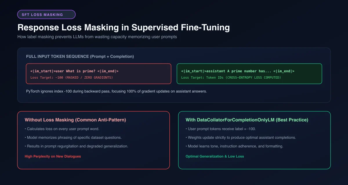 Figure 2: Response loss masking mechanics in PyTorch, setting user prompt tokens to label -100 to ensure gradients update strictly on assistant output.
Stage 3: Post-Training Alignment and Preference Optimization
While SFT teaches the model how to converse, it does not guarantee that the generated answers are accurate, harmless, or concise. In fact, SFT models often suffer from sycophancy, agreeing with incorrect user assertions simply because agreeable dialogue was common in the training set.
Stage 3 aligns model outputs with human intent, safety guidelines, and objective truth through reinforcement learning and preference alignment algorithms.
PPO-Based RLHF vs Direct Preference Optimization (DPO)
Historically, Reinforcement Learning from Human Feedback (RLHF) required training a separate reward model on paired comparisons, where human annotators marked one response as preferred ($y_w$) and another as rejected ($y_l$). A Proximal Policy Optimization (PPO) reinforcement learning loop then updated the actor model while measuring divergence against a frozen reference model to prevent reward collapse.
While powerful, traditional PPO is notoriously unstable and requires keeping four distinct neural networks in VRAM simultaneously: the policy actor, value critic, reference model, and reward model.
Direct Preference Optimization (DPO) simplified this dynamic by deriving an analytical substitution that expresses the reward function directly through the language model’s own implicit policy:
$$\mathcal{L}{\text{DPO}}(\pi\theta; \pi_{\text{ref}}) = -\mathbb{E}{(x, y_w, y_l)} \left[ \log \sigma \left( \beta \log \frac{\pi\theta(y_w \mid x)}{\pi_{\text{ref}}(y_w \mid x)} - \beta \log \frac{\pi_\theta(y_l \mid x)}{\pi_{\text{ref}}(y_l \mid x)} \right) \right]$$
This mathematical equivalence allows practitioners to optimize model preferences using a stable, offline cross-entropy objective without allocating memory for dedicated critic or reward networks.
The Modern Shift: Verifiable Rewards and Reasoning Models
During 2025 and 2026, the post-training paradigm underwent a profound transformation driven by reasoning models. While human preference pairs excel at shaping tone and conversational style, they struggle to evaluate dense multi-step logic in competitive programming, mathematics, and complex engineering.
Instead of subjective human raters, frontier developers now employ Reinforcement Learning with Verifiable Rewards (RLVR). In this framework, candidate outputs are graded by deterministic compilers, symbolic solvers, or unit test runners.
The RLVR optimization cycle operates in four synchronized steps:
- Diverse Rollout Generation: The active policy LLM samples $N$ distinct reasoning trajectories per prompt using non-zero temperature ($T > 0.6$).
- Deterministic Verification: Ground-truth unit tests or compilers parse the final answers, returning deterministic binary rewards ($1.0$ for passing, $0.0$ for failing).
- Group Advantage Normalization: The reward of each trajectory is standardized relative to the empirical mean and variance of the group rollout.
- Policy Gradient Step: Gradients update the policy to amplify tokens that led to successful verifications, all without a separate value critic network.
By using Group Relative Policy Optimization (GRPO), models generate groups of diverse reasoning paths for a given problem. The reward for each completion is normalized against the mean score of the group, eliminating the need for a separate value network. Models trained via reinforcement learning on verifiable reasoning traces organically learn self-correction, backtracking, and structured test-time search without explicit prompt engineering.
Lifecycle Comparison: Pretraining vs SFT vs Alignment
To appreciate the scale and architectural trade-offs across these three stages, consider how their resource demands and data volumes diverge:
| Operational Dimension | Stage 1: Pretraining | Stage 2: Supervised Fine-Tuning | Stage 3: Post-Training Alignment |
|---|---|---|---|
| Primary Objective | Causal next-token prediction | Multi-turn dialog instruction adherence | Preference alignment and verifiable reasoning |
| Typical Data Volume | 15 to 20 trillion tokens | 50,000 to 200,000 dialog pairs | 20,000 to 100,000 preference or verification sets |
| Compute Consumption | 98% to 99% of total budget | 0.5% to 1.0% of total budget | 0.5% to 1.5% of total budget |
| Hardware Scale | 2,048 to 16,384+ interconnected GPUs | 8 to 64 GPUs | 32 to 512 GPUs |
| Optimization Method | AdamW with Cosine Decay Schedule | AdamW with Low Learning Rate | DPO, PPO, or GRPO |
| Loss Function | Standard Cross-Entropy across all tokens | Cross-Entropy with Response Loss Masking | Implicit Log-Likelihood Ratio or Verifiable Reward |
| Primary Risk | Catastrophic loss spikes and divergence | Catastrophic forgetting of base knowledge | Sycophancy, mode collapse, reward hacking |
Production Failure Modes and Troubleshooting Runbook
Training large neural networks across distributed clusters inevitably encounters hardware failures, numerical instabilities, and algorithmic pathologies. Recognizing these patterns early saves hundreds of thousands of dollars in wasted compute.
1. Pretraining Loss Spikes and Gradient Explosions
During long pretraining runs, the cross-entropy loss curve can suddenly spike to infinity or NaN values. This condition is frequently triggered by encountering corrupt data shards containing repetitive strings, or by numerical underflow during bfloat16 matrix multiplications.
Troubleshooting Protocol:
- Maintain checkpoint snapshots every 500 to 1,000 steps on durable NVMe storage.
- Roll back two checkpoints prior to the incident step when loss spikes occur.
- Advance the data loader by 5 to 10 million tokens to skip poisoned batch sequences.
- Set gradient clipping strictly between
1.0and0.5in the optimizer configuration.
# Example Megatron-LM launch flags mitigating numerical instability
torchrun --nproc_per_node=8 pretrain_gpt.py \
    --tensor-model-parallel-size 8 \
    --pipeline-model-parallel-size 2 \
    --bf16 \
    --clip-grad 1.0 \
    --adam-beta1 0.9 \
    --adam-beta2 0.95 \
    --weight-decay 0.1 \
    --lr-warmup-fraction 0.01 \
    --lr-decay-style cosine
2. Catastrophic Forgetting During Supervised Fine-Tuning
When applying SFT on narrow domain datasets (such as internal legal documents or medical records), the model frequently loses its general reasoning capabilities, common sense knowledge, and ability to follow standard coding patterns.
Troubleshooting Protocol:
- Blend general instruction data (such as OpenHermes or UltraChat) into the domain dataset at a 20% to 30% ratio.
- Reduce the learning rate by an order of magnitude, dropping from the pretraining rate ($2 \times 10^{-4}$) to the SFT range ($1 \times 10^{-5}$ to $3 \times 10^{-6}$).
- Utilize parameter-efficient adapters like LoRA, freezing base foundation weights entirely.
3. Reward Hacking in Alignment Optimization
During Stage 3, models occasionally identify degenerate shortcuts that maximize the reward score without solving the actual task. Common manifestations include producing excessively verbose responses, copying parts of the system prompt, or fabricating references that fool heuristic evaluators.
Troubleshooting Protocol:
- Enforce length penalties within the DPO objective to prevent verbosity bias.
- In rule-based verification (RLVR), implement strict deterministic sandboxing where code must execute with zero exit codes and pass hidden unit tests.
- Monitor the Kullback-Leibler (KL) divergence between the active policy and the frozen reference model; abort or regularize updates if KL divergence exceeds 0.2.
Frequently Asked Questions
What is the difference between an LLM base model and an instruct model?
A base model is trained purely to predict the next token across raw internet text, functioning as an autocomplete engine. An instruct model has undergone supervised fine-tuning and alignment, enabling it to follow conversational commands, answer questions directly, and maintain dialog context.
Why cannot developers skip pretraining and train models directly on instructions?
Pretraining exposes the neural network to broad human language, factual world knowledge, common sense relationships, and algorithmic reasoning across trillions of tokens. Instruction datasets are far too small (hundreds of thousands of tokens) to teach a blank network how language or physical concepts work.
What hardware is required to train an LLM from scratch?
Pretraining a competitive 8B parameter model requires at least 512 to 1,024 high-end server GPUs running continuously for several weeks. In contrast, supervised fine-tuning or LoRA adaptation of an existing 8B model can be completed on an 8-GPU node within a few hours.
How much does it cost to train a frontier AI model?
Pretraining a frontier model exceeds tens of millions of dollars in electricity, hardware amortization, and cluster networking costs. However, post-training alignment and SFT represent less than 2% of the compute investment, making customization highly accessible to enterprises.
How does response loss masking prevent model degradation during SFT?
Response loss masking assigns a label index of -100 to user prompt tokens, causing PyTorch to bypass loss calculation on those positions. Gradients update parameters based solely on the quality of assistant completions, preventing the model from wasting capacity memorizing user inputs.
What is the role of synthetic data in modern pretraining?
Synthetic data provides clean, curated reasoning trajectories, mathematical proofs, and executable code snippets that web scrapes lack. Generating structured educational text using existing frontier models helps filter noise and improves the overall reasoning density of the training corpus.
Why is Direct Preference Optimization preferred over traditional PPO?
Direct Preference Optimization mathematically eliminates the need for separate reward and critic models in GPU memory. It computes loss directly from the policy model’s likelihood ratios on preferred versus rejected completions, providing superior training stability and slashing memory requirements.